Clearing Kidney Exchanges via Graph Neural Network Guided Tree Search
- 14 minsLast summer, I researched the application of Graph Neural Networks (GNNs) to the Kidney Exchange under the guidance of Professor John Dickerson. This approach used deep learning to discover heuristics to approximate solutions to the kidney exchange. Specifically, these heuristics represent tradeoffs between conflicting Kidney Exchange configurations. I trained a GNN on a dataset of solved kidney exchanges, and then used a tree search to refine the output of the GNN. This project won the ACM/CSTA Cutler-Bell Prize in High School Computing, was presented at the AAAI Student Abstract Poster Session, and will be published in the AAAI 2020 proceedings.
Background
The kidney exchange was developed to help incompatible patient-donor pairs get compatible kidneys.
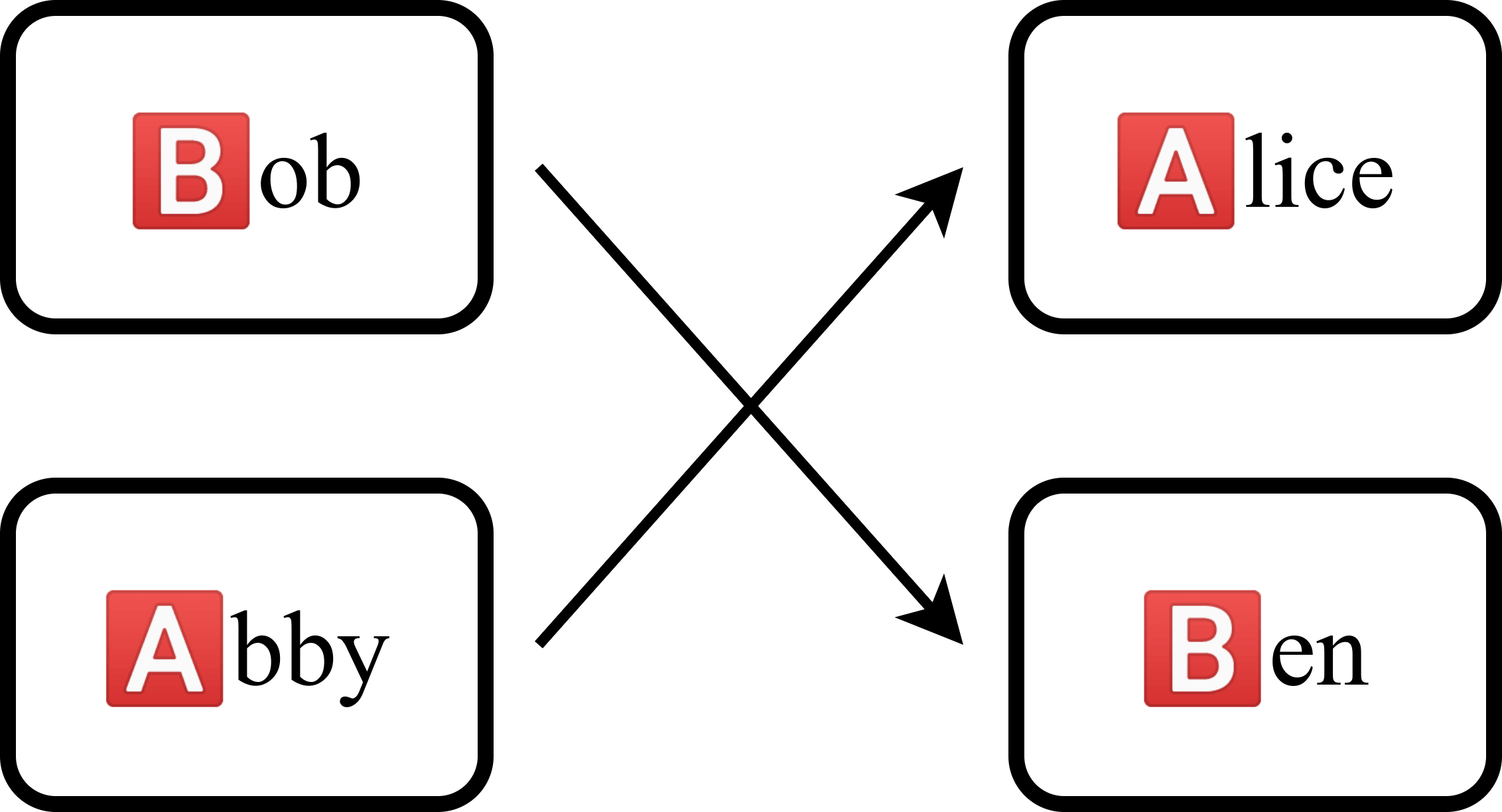
Suppose we have a patient, Alice, and a donor, Bob. Alice has type 🅰️ blood while Bob has type 🅱️ blood. For the sake of demonstration, let us assume that only blood type determines compatibility. So currently, Bob cannot donate to Alice.

Meanwhile, we have another patient-donor pair, Ben and Abby, with blood types 🅱️ and 🅰️ respectively. Once again, Abby cannot donate to Ben because of their incompatible blood types.

What if we were to link the two groups together, having Bob donate to Ben and Abby donate to Alice? Now, two initially incompatible groups can leave with donations.

Another way of representing the situation is to use a compatibility graph. In a compatibility graph, the nodes represent patient-donor pairs while the arrows represent compatibility. An arrow connects from one pair to another pair if the former’s donor can donate to the latter’s patient.
This is the compatibility graph representation of the first example:

Notice that this configuration forms a 2-cycle. We can generalize to n patient donor pairs: if the donor of one pair is compatible with the patient of the next, we can daisy-chain all of these donors.
This is the crux of the Kidney Exchange: to pool together incompatible patient-donor pairs so that they can leave with transplants.
Cycle Conflicts and Practical Issues
With just two “mutually-compatible” pairs, everything runs smoothly. However, when there are pairs, we may run into trouble. Below, we have a four pair pool:
There are two cycles in this pool. However, these two cycles cannot coexist. Each kidney donor can only donate one kidney (and any pair donating expects one in return). For both cycles to work, the donor of pair [B] has to donate to the patients of [C] and [A], which is not possible! Thus, we have to choose between the cycle on the left or right. We denote that these two cycles are incompatible.
Such conflicts occur often in large pools. To resolve them, we need a way to quantify how valuable a cycle is. In practice, variables include the number of patients saved, the probability of success, and perhaps social values (fairness objectives). Combining the number of patients saved and their probabilities, we arrive at the expected number of patients saved.
In our model, we give equal weight to each patient and their chance of success. We also limit ourselves to cycles sizes less than 5, as most hospitals only have enough resources to handle 5 pairs (shorter cycles generally have greater success, too). That is, we maximize the number of patients saved, subject to a size restriction of 5.
So, in the two cycle example above, we will choose the left cycle of size three over the right cycle of size 2.
Resolving these conflicts can be thought of as a Weight Maximum Independent Set problem (WMIS). The WMIS problem is NP-hard, and current state of the art approaches require exponential time to solve it exactly.
Deep Learning
We use a Graph Neural Network (GNN) to find solutions to these conflicts. Specifically, the GNN’s job is to predict which of the cycles present in the pool are optimal while respecting the constraints of cycle compatibility.
A key assumption we make is that real world Kidney Exchanges conform to an underlying data distribution. That is, the Kidney Exchange compatibility graphs we see might be similar: each graph may contain different variations, but they share an underlying structure. For example, there could be certain motifs or patterns that occur often in these graphs. Instead of solving these graphs anew with an off-the-shelf solver like Gurobi, we would like to develop heuristics to exploit this structure.
GNNs run in polynomial time and excel at operating on structured graphical data, so we believe this architecture could help us build a quick approximation to the Kidney Exchange WMIS problem. Unlike traditional Convolutional Neural Networks, GNNs can adapt to a variety of graph sizes, scaling up or down due to their special convolutions.
We build a pipeline to transform our Compatibility Graph into a new form of what we call a WMIS graph. In the WMIS graph, the nodes are cycles in the compatibility graph and the edges represent incompatibility between cycles. The weight of each vertex represents the number of patients covered by its Compatibility Graph cycle. Since we would like to maximize the number of patients matched, we would like to maximize the sum of all the weighted vertices in the WMIS graph. This new format makes it possible for our GNN to operate effectively.
In summary, our Graph Neural Network is designed to figure out what cycles are optimal (lead to the greatest weighted sum) given a WMIS graph. It indicates the good cycles with a high probability (close to 1) and poor cycles with a low probability (close to 0). These probabilities do not need to be normalized (sum to 1) because multiple cycles can exist. However, we would like these cycles to respect constraints of the WMIS graph, the rule that two neighbors should not have high probabilities.
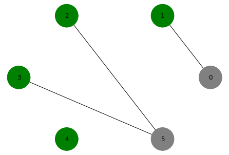
Below, we have a diagram of what a GNN could output. The graph itself is a compatibility graph, while the green bars represent beliefs that the GNN predicts.
As you can see, the middle vertex in this diagram is assigned a relatively low probability (it has “too many neighbors” to affect), while another has almost a full bar (it is quite isolated). The graph neural network, through its convolutions and layers, is able to be trained to figure out these quantities.
Graph Neural Network Model
We adopt a standard architecture for our Graph Neural Network (GNN). Below is a diagram summarizing the architecture of our GNN.
The network’s input would be a WMIS graph, which consists of nodes, node’s weights and edges. The input is then passed through several convolution layers. After doing several experimental trials, we settled on using the GNN operator GraphConv from the PyTorch Geometric library. Between each graph convolution is a ReLU unit, which introduces non-linearity into the network. The graph convolutions are defined mathematically as follows:
The graph convolutional layers differ by the aggregation functions used. In the summary diagram, we see that some layers have max aggregations while others have additive aggregations. These two aggregations are inspired by the max-sum belief propagation algorithms used for probabilistic belief inference. Also, we found empirically that this architecture delivers good performance.
The final layer of this graph neural network is a fully connected layer. This layer ensures that the result is a valid probability map, that each node’s value is between zero and one.
Training
We created a dataset of randomly generated compatibility graphs and their solved counterparts for our GNNs to train on. The comparability graphs were generated according to the Erdos-Renyi model, and we randomly assigned weights to each node. Then, we formulated the WMIS problem for each compatibility graph as an Integer Linear Program (IP Program). To solve these IP programs to optimality, we used Gurobi, a commercial optimization solver.

With a dataset and its corresponding labels in hand, we trained the GNN by minimizing the binary cross-entropy loss between the GNN output and the optimal labels computed by Gurobi. This approach could run into problems as a single compatibility graph may have multiple optimal solutions. The GNN may output an optimal solution but be “corrected” by the dataset. Also, one can imagine that the GNN could be torn apart by several optimal solutions, as even two identical compatibility graphs may have completely different solutions. This would cause the GNN to spread its probabilities across different solutions (and therefore nodes), weakening its power to identify good compatibility graph nodes. We are currently still working on this issue, and we plan by introducing different loss functions (perhaps Reverse KL) to correct this behavior.
Training Results
After training our GNN on the dataset solved by Gurobi, we obtained a well performing GNN. Below are the graphs detailing cross entropy losses over training epochs:
We see that the GNN is able to generalize to unseen instances as shown by the validation loss graph.
Tree Search
Now, we have a working GNN that predicts promising cycles. We would like to improve predictions by using a search algorithm to search other plausible compatibility graph configurations.
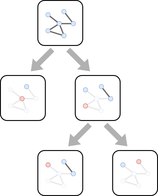
First, we need to specify the overall framework of the search space. The WMIS problem can be thought of as an iterative and recursive problem. We begin with the original compatibility graph, and to pick a node, we remove it and all its neighbors. The residual graph left behind is another WMIS problem, a smaller subproblem.

Since the general WMIS problem is NP-hard, it is unlikely that a WMIS problem for compatibility graphs could be solved by brute force enumeration. We would like a way to narrow down our search to something more reasonable. To do so, we leverage the GNN’s predictions to help find promising branches.
One way to incorporate GNN’s predictions into searches is to use a heuristic search algorithm. The specific search algorithm we use is a variant of the Monte Carlo Tree Search algorithm. The search algorithm, like the GNN, seeks to identify which vertices in the compatibility graph are valuable. However, instead of returning a fully probability map, this search algorithm would just return only the promising vertex.
The Monte Carlo Tree Search algorithm consists of four key steps that are run repeatedly: Selection, Expansion, Simulation and Backpropagation.
During the selection phase, the Monte Carlo Tree Search recursively iterates through the different search nodes, picking the most promising branch at each stage by assessing the search nodes’ combined Q and U scores:
\[\DeclareMathOperator*{\argmax}{arg\,max} a_t = \argmax_{a}(Q(s_t, a) + U(s_t, a))\]The U score represents a combination of an exploration factor and the GNN’s assessment. The exploration factor decreases as the branch is explored more; this incentivizes the algorithm to search less explored areas. The U score also incorporates information from the GNN. Through the GNN’s probability map, we can estimate each node’s value. The U score acts like a prior, allowing the search algorithm to incorporate knowledge from the GNN.
\[U(s_t, a) = c * P(s_t, a) * \dfrac{\sqrt{\sum_{b}N(s_t, b)}}{1 + N(s_t, a)}\]The Q score is a statistic tracked by the search algorithm itself, and will be explained in the later sections. For now, you could think of this Q function as a Q function in Reinforcement Learning: the expected value of the graph, or the sum of nodes in a valid WMIS configuration.
Selection phase ends when the algorithm hits a leaf node. During the expansion phase, we expand the tree by incorporating a new state generated from a leaf node.
Then, we estimate the value of the newly expanded state during the simulation phase. We greedily pick nodes and repeatedly remove its neighbors until the graph becomes empty. This generates a valid maximal independent set. We view this maximal independent set as a lower bound on the value of the state; the performance can only improve with a better selection.
After the simulation phase, the obtained value from the greedy sample is backpropagated through the various Q values of the parent nodes. When updating, we use a max operator, as each sample can be viewed as a lower bound, as stated above.
Experiments
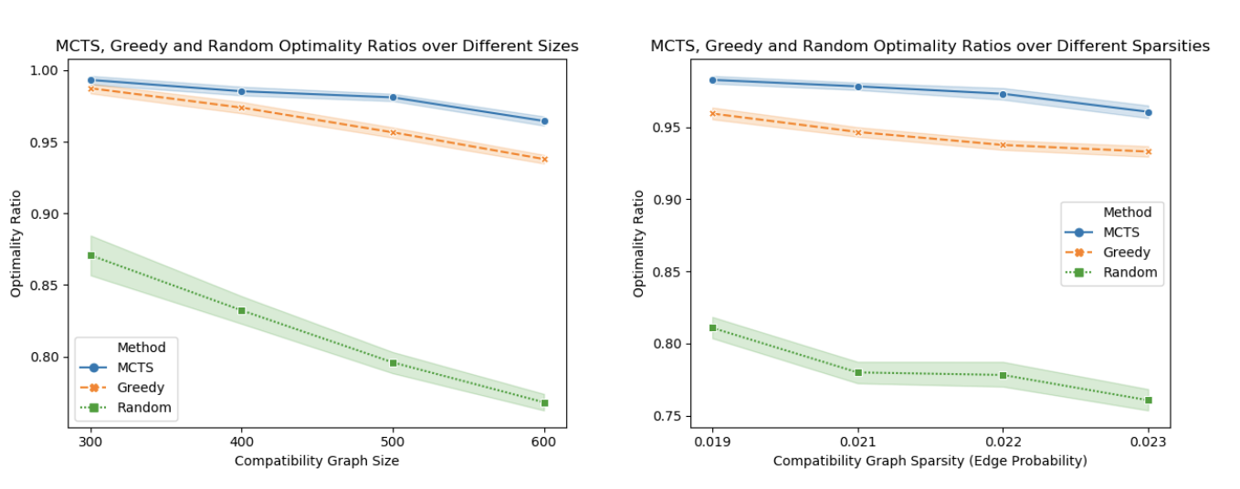
With the combined GNN and tree search algorithm, we can squeeze out even more performance. We tested our algorithm on a newly generated set of Erdos-Renyi Compatibility graphs with two varying parameters: graph size and graph sparsity. Graph size is just the number of nodes in the graph, while sparsity specifies the probability of an edge between any two nodes. In a denser graph, we expect much more cycles, and thus, a harder problem (there will be more vertices the corresponding WMIS problem).
We evaluate our algorithm against two baselines: random and greedy. Random generates a valid Maximal Independent Set (MIS) by iteratively picking a random node, while greedy iteratively picks the node with the smallest neighbor sum (sum of all the weights of the neighbors).
Instead of Cross-Entropy Loss, we use the optimality ratio to measure the performance of our combined tree search algorithm. The optimality ratio is defined as algo_score/optimal_score, where the algo_score is the number of patients matched by the algorithm, while optimal_score is the optimal number of patients matched (computed by Gurobi). 
As shown in the graph, our algorithm outperforms baselines by a large margin for a variety of sizes and sparsities. The shaded area of the lines are 95% confidence intervals. None of our algorithm’s CIs overlap with the baselines, so we are confident that our algorithm outperforms the baselines under these conditions.
Further Reading
Although this post gives an in-depth summary of my research, you may be still curious about some of the details of my algorithms. If you would like to learn more about these technical details, you could check out my AAAI research paper and code repository (still a work in progress, especially the documentation).
I have also created a video, a presentation and a poster. For more in depth resources about Graph Neural Networks I recommended these links:
Monte Carlo Tree Search Resources:
I learned a great deal from these and many other resources, and I appreciate the ML community for taking their time to illuminate concepts for others.


